Stock Valuation

In this post, I will explain some methods of valuating stock prices. If we show the Free Cash Flow of this company at year $n$ from now by $\textrm{FCF}_n$ and if the discount rate is $r$, then the Present Value of Future Free Cash Flows (PVFFCF) of the company will be equal to

However, it is not possible to estimate cash flows forever so we need to estimate cash flows for a growth period and then estimate a Terminal Value of Future Free Cash Flows (TVFFCF), to capture the value at the end of the period. Assume that the company enters the maturity period at the end of year $N$, then the Present Value of Future the company can be estimated as

One way to estimate the terminal value is to use the stable growth model or perpetuity growth model or Gordon growth model or Dividend Discount Model (DDM). In this model, we assume that when the comany enters its mature phase of operations, its free cash flow grows at a constant rate of $g$. We assumed that the company just entered the maturity phase at the end of year $N$, so we can say that the company’s free cash flow at year $N+i$ for $i=1,2,…$ will be equal to

Since want to calculate the terminal value at the beginning of the maturity phase, we need to discount $\textrm{FCF}_{N+i}$ to the end of year $N$. Therefore, we have

Notice that the assumption is that the overall economy is composed of high growth and stable growth firms and therefore the growth rate of the latter is less than the average growth rate of the economy. Therefore, in the above formula the stable growth rate $g$ should be set smaller than the discount rate $r$. However, $g$ can be negative implying that the firm is losing value over time.

Finding $\textrm{TVFFCF}$ enables us to find $\textrm{PVFFCF}$. We can then subtract the company’s Total Debt (DEBT) from $\textrm{PVFFCF}$ and add the sum of Cash and Cash Equivalents (CASH) to it to find the Equity Value (EQUITY) of the company.

The stock price of the company is then found by dividing the equity value by the Number of Shares Outstanding (SHARES)

To be able to use the above method, we need to be able to have good estimates for $\textrm{FCF}_i$ for $i=1,2,…,N$. On top of that, it is also very important to choose the right estimates for $r$ and $g$. The more accurate estimates we can find for these values the more accurate our stock valuation will become.

As a simple first step, we can look at the previous FCF values and try to fit a linear least squares model to this data and predict the future FCFs. Assume that we look at the past $m$ years of company FCF data and let the FCF at year $x_t$ for $t = t_0, t_0 -1,…, t_0 - (m-1)$ be denoted by $y_t$ and let the predicted least squares value of FCF at year $t$ be $\hat{y}_t = a x_t + b$. Miniming the square error using linear least squares we can easily show that if we denote:

Then

and

We can then use the estimated parameters to estimate $\textrm{FCF}_i$ as \(\hat{y}_{i} = a x_i + b\) for $i = 1,2,…, N$.

For estimating the discount parameter $r$, we need to find the Weighted Average Cost of Capital (WACC) or Cost of Capital for the firm that we analyzing. WACC is the average rate that the company is required to pay to its debt holders, investors and other types of financiers. This rate is dictated by the market and if the firm is not able to pay that rate, the financiers would seek better opportunities. In general, WACC can be quite complex to find as the firm may have many different financiers with different rates. However, in cases when the firm is only financed with debt and equity, we have

In the equation above Cost of Equity is the return that the firm theoretically pays to its equity investors, i.e., shareholders, to compensate for the risk they undertake by investing their capital. It can be calculated using the $\beta$ parameter in CAPM as

where $r_f$ is the risk-free return which can typically be found from government bond yields and $r_m$ is the historical return of the stock market and $\beta$ is a unique parameter for the firm found through CAPM.

Cost of Debt on the other hand shows the interest rate that the company is paying on its borrowed funds. It can be calculated as

where $r_f$ is the risk-free return, $T$ is the firm’s tax rate and credit spread is the difference between the rate that corporate bonds are paying compared to gonvernment bonds. Firms with lower credit rating have higher credit spreads which means that they are more risky and they need to pay higher returns to be able to borrow money from the open market. Notice that cost of debt is expressed as an after tax rate because the interest deductible for income taxes to allow for fair comparisons. That’s why the above equation includes a tax term. Summarizing above, if we show the debt to equity ratio by $D/E$ then the discount rate to be used in our stock valuation formula will be found as

The last peice of our stock valuation puzzle is the parameter $g$ which is the stable growth rate. One way of estimating this value is to look at the average growth rate of the stable firms in that industry branch and use it as a proxy for $g$.

Example

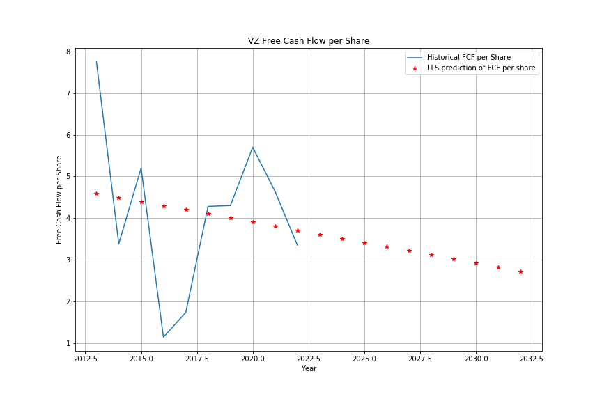
Let’s analyze the value of a few stocks say Nvidia with ticker NVDA and Verison with ticker VZ using this method. We can get the past $m=10$ years of FCF data for VZ from this link and for NVDA from this link. To simplify our analysis, we work with Free Cash Flow per Share data, i.e. the last line of data in these links. Writing a few lines of code in Python, we can estimate and plot the next $N=10$ years of FCF values as follows.

import numpy as np
import matplotlib.pyplot as plt

years = list(range(2013, 2023))
futures = list(range(2023, 2033))
fcf_share = {
    "NVDA" : [0.26, 0.36, 0.51, 0.69, 1.22, 1.29, 1.75, 1.9, 3.26, 1.53],
    "VZ": [7.75, 3.38, 5.20, 1.14, 1.73, 4.28, 4.30, 5.70, 4.64, 3.35]
}

def find_lls_params(ticker):
    n = len(years)
    mx = np.mean(years)
    mxx = np.mean([x**2 for x in years])
    denom = mxx - mx**2
    b = (np.mean([years[i]*fcf_share[ticker][i] for i in range(n)]) -  np.mean(fcf_share[ticker]) * mx)/denom
    c = np.mean(fcf_share[ticker]) - b * mx
    return b, c

def find_lls_points(ticker):
    b, c = find_lls_params(ticker)
    data = {x:b*x+c for x in years+futures} 
    return data

def plot_lls_points(ticker):
    plt.figure(figsize=(12,8))
    plt.plot(years, fcf_share[ticker])
    lls_data = find_lls_points(ticker)
    plt.plot(lls_data.keys(), lls_data.values(), 'r*')
    plt.grid()
    plt.legend(['Historical FCF per Share', 'LLS prediction of FCF per share'])
    plt.ylabel('Free Cash Flow per Share')
    plt.xlabel('Year')
    plt.title(ticker +' Free Cash Flow per Share')
    return lls_data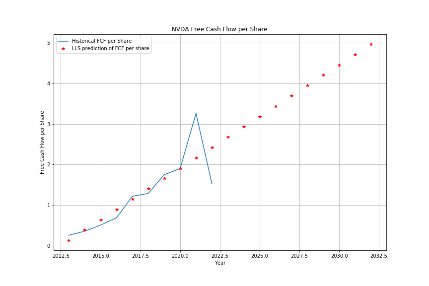

Now, it remains to estimate the discount rate for these stocks. There are certain websites that have these rates calculated for us. For instance, WACC for VZ can be found from here and for NVDA from here. However, we can also calculate these values using the formulas above. For instance, we can find risk-free interest rates from this website and values of $\beta$ from here and here and we can use any stock charting website to calculate the historical value of $r_m$ for the overall market. This allows us to confirm that the WACC numbers in the above links actually make sense.

Taking the values of selected WACCs in the links above and assuming that NVDA has a stable growth rate of 4% and VZ has a stable growth rate of 4% then PVFFCF per share will be caculated to 76.84 and 105.88, respectively. I used the following peice of code for that calculation:

def calculate_PVFFCF(lls_data, r_wacc, g):
    N = len(futures)
    TVFFCF_share = lls_data[futures[-1]]*(1+g)/(r_wacc-g)
    PVFFCF_share = TVFFCF_share / (1+r_wacc)**N
    for year in futures:
        i = year - years[-1]
        PVFFCF_share += lls_data[year] / (1+r_wacc**i)
    return PVFFCF_share

Now, we need to look at the values of debt and cash assets for these two companies. These numbers can be found from links like this for NVDA and this for VZ. If we subtract total debt from cash and cash equivalents that we have from these links and divide that by the number of outstanding shares that we can find from here for NVDA and here for VZ and if we add that ratio to the PVFFCF per share numbers we found above, then we can find the estimate for stock price. In this case, it leads to a stock price of 77.42 for NVDA and 64.5 for VZ on April 30th 2023. We can see that these values are inline with the values found here for NVDA and here for VZ with 10 year growth exit number. This implies a sell on NVDA and a buy on VZ based on respective current prices of 277.49 and 38.83.