Upper Confidence Bound algorithm in Multi-Armed Bandits

In this post, I will try to explain some interesting ideas around multi-armed bandits. I will implement the greedy exploitation algorithm along with the Upper Confidence Bound algorithm in Python for a simple multi-armed bandit problem.

import numpy as np
import math 
import matplotlib.pyplot as plt

Defining a simple multi-armed bandit as follows

def multiArmedBandit(k):
    if k == 0:
        return 2*np.random.randn()+1
    elif k == 1:
        return np.random.randn()+2
    elif k == 2:
        return 3*np.random.randn()
    elif k == 3:
        return np.random.uniform(-5,5)
    else:
        return None

It is clear that arm 1 has the largest expected value of reward which is equal to 2. Hence, the optimal value v* is equal to 2. This value will be used to compute the regret. Also we have

q(0) = 1 => regret = 1
q(1) = 2 => regret = 0
q(2) = 0 => regret = 2
q(3) = 0 => regret = 2

The following piece of code can be used to plot the distribution of different arms

N = 100000 
arm0 = [multiArmedBandit(0) for _ in range(N)]
arm1 = [multiArmedBandit(1) for _ in range(N)]
arm2 = [multiArmedBandit(2) for _ in range(N)]
arm3 = [multiArmedBandit(3) for _ in range(N)]
bins = np.linspace(-10, 10, N/500)
plt.figure(figsize=(14,4))
plt.hist(arm0, bins, alpha=0.5, label='arm 0')
plt.hist(arm1, bins, alpha=0.5, label='arm 1')
plt.hist(arm2, bins, alpha=0.5, label='arm 2')
plt.hist(arm3, bins, alpha=0.5, label='arm 3')
plt.legend(loc='upper right')
plt.show()

This is a histogram of the distribution of different arms Arm distributions This plot clearly shows that the best action to take would be action 1 which is equivalent to taking the second arm. However, this distribution is unkown to the agent and therefore, they cannot choose the optimal action. But they can try to sample from different actions. If they follow a greedy approach as below

def full_exploitation(t):
    # Greedy approach: full exploitation and no exploration 
    A = [multiArmedBandit(i) for i in range(4)]
    max_idx = max(range(4), key=lambda i:A[i])
    #print("arm0 :{:.2f}  arm1 :{:.2f}  arm2 :{:.2f}  arm3 :{:.2f}\t ==> Selected Arm: {}".format(\
    #    A[0], A[1], A[2], A[3], max_idx))
    qa = [1, 0, 2, 2]
    regrets = [qa[max_idx]]*t
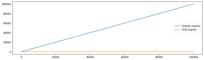
    return [multiArmedBandit(max_idx) for _ in range(t)], regrets, [max_idx]*t

Then, the regret bound grows linearly with time t but if they follow the Upper Confidence Bound algorithm as

def ucb_algorithm(t):
    assert t>3, "t should be greater than the number of arms"
    counts = {i:[multiArmedBandit(i), 1] for i in range(4)}
    rewards = [counts[i][0] for i in counts]
    actions = [0,1,2,3]
    qa = [1, 0, 2, 2]
    regrets = [1, 0, 2, 2]
    for step in range(4, t):
        C = [counts[k][0] + math.sqrt(2*math.log(step)/counts[k][1]) for k in counts]
        action = max(range(4), key=lambda i:C[i])
        actions.append(action) 
        rewards.append(multiArmedBandit(action))
        counts[action][1] += 1
        counts[action][0] += (rewards[-1]-counts[action][0])/(counts[action][1])
        regrets.append(qa[action])
    return rewards, regrets, actions

then the regret bound increases logarithmically with t. Here is the code to see the results,

def compute_list_cumulative(A):
    if len(A) < 1: 
        return []
    B = [A[0]]
    for i in range(1, len(A)):
        B.append(B[-1] + A[i])
    return B

T = 100000
steps = list(range(1, T+1))
ucb_rewards, ucb_regrets, ucb_actions = ucb_algorithm(T)
greedy_rewards, greedy_regrets, greedy_actions = full_exploitation(T)
greedy_regrets_cumul = compute_list_cumulative(greedy_regrets)
ucb_regrets_cumul = compute_list_cumulative(ucb_regrets)
plt.figure(figsize=(14,4))
plt.plot(steps, greedy_regrets_cumul, label = 'Greedy regrets')
plt.plot(steps, ucb_regrets_cumul, label = 'UCB regrets')
plt.legend(loc='right')
plt.show()

And this plot shows the regret bounds. A summary of this code is available in this notebook.