Gradient Bandits

In this post, I will explain the fundamentals of gradient bandits. First, I will explain the Log-likelihood trick (or REINFORCE trick, Williams 1992). Assume that $\theta$ is the parameter vector and $R_t$ is the reward at time t which is a function of $\theta$. Also, let $A_t$ be the action at time t, $\pi_{\theta}(a)$ be the policy which is parametrized on $\theta$ and we want to find it directly through gradient updates. Letting

and running gradient ascent on parameters $\theta$ to maximize the expected reward, we have

However, this is not quite possible since we need to first take the average and then take the gradient. We cannot simply do the sampling. Hence, we can write the second term as

This allows us to easily perform stochastic gradient descent since now we are sampling from the values of the gradient. In this case, the stochastic gradient update formula looks like

The policy can be a very complex function and it can be a deep network as we know how to compute gradients on deep networks. This is what makes this approach unique. We only need to sample the reward and its corresponding action for each iteration of the gradient ascent algorithm.

In the following, we will use this trick to derive the gradient update equation for the case of softmax policy preferences (derivation from Richard Sutton). If $H_t(a)$ shows the action preference in a softmax setting we have,

Gradient ascent updates the preference as

where the expected reward is computed as

hence,

Where $B_t$ called the baseline, can be any scalar that does not depend on $x$. The baseline can be included without changing the equality because the gradient sums to zero over all the actions, $\sum_x \frac{\partial \pi_t(x)}{\partial H_t(a)} = 0$. As $H_t(a)$ is changed, some actions probabilities go up and some go down, but the sum of the changes must be zero because the sum of the probabilities is always one. If we multiply each term of the sum by $\frac{\pi_t(x)}{\pi_t(x)}$, we have

The equation is now in the form of an expectation, summing over all possible values $x$ of the random variable $A_t$, then multiplying by the probability of taking those values, we have

Noting that $q_{\star}(A_t) = \mathbb{E}[R_t | A_t]$ and choosing $B_t = \bar{R}_t$ where $\bar{R}_t$ is the average of all the rewards up through and including time $t$, we have

Using equation \eqref{eq_def_pi} we can prove that

Hence,

Now that we wrote this in the form of a nice expectation, we can sample in each step and therefore, we can write the update equation for stochastic gradient ascent algorithm as

This equation can be written as

This means that we select a certain action and we update all the preferences. The algorithm updates all action preferences in each step. The $\bar{R}_t$ term serves as a baseline with which the reward is compared. If the reward is higher than the baseline, then the probability of taking $A_t$ in the future is increased, and if the reward is below baseline, then probability is decreased. The non-selected actions move in the opposite direction. The baseline helps reduce the varaince.

Here is a simple Python implementation of this algorithm (inspired by this post).

import numpy as np
import math
import matplotlib.pyplot as plt

def get_rewards():
    mean = np.array([-2, 1, 0, -3]) 
    return np.random.randn(4) + mean

def softmax(H):
    h = H - np.max(H)
    exp = np.exp(h)
    return exp / np.sum(exp)

def gradient_bandit(N):
    H = np.zeros(4)  
    r_hist = []
    alpha = 0.1  
    for t in range(1, N):
        policy = softmax(H) # policy pi
        # sampling (choice) action by policy
        a = np.random.choice(4, p=policy) 
        rewards = get_rewards()
        r = rewards[a] # R_t (reward for chosen action)
        r_hist.append(r)
        avg_r = np.average(r_hist)
        # update a == A_t (chosen action)
        H[a] = H[a] + alpha*(r-avg_r)*(1-policy[a])
        # update a != A_t (non-chosen action)
        H[:a] = H[:a] - alpha*(r-avg_r)*policy[:a]
        H[a+1:] = H[a+1:] - alpha*(r-avg_r)*policy[a+1:]
    
    return softmax(H), r_hist

opt_policy, r_hist = gradient_bandit(100)
plt.plot(opt_policy, 'o')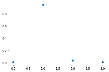

A summary of this code is available in this notebook.