Notes on Optimal Transport
This post is dedicated to optimal transport. I will summarize the fundamentals of optimal transport in this page. Mainly, I will summarize the nice survery Computational Optimal Transport along with talks by Marco Cuturi.
Monge Problem
The study of optimal transport first started by Monge in 1781 by trying to find a deterministic mapping $T(.)$ that can optimally transport all the mass in one space to another space. More formally, assuming that we have arbitrary probability measures $\alpha$ and $\beta$ on respective spaces of $\mathcal{X}$ and $\mathcal{Y}$, then Monge’s problem is to find a mapping $T: \mathcal{X} \to \mathcal{Y}$ that minimizes
\[\min_{T} \left\{ \int_{\mathcal{X}} c(x, T(x)) \mathrm{d} \alpha(x) ~~:~~ T_\sharp \alpha = \beta \right\}\]where $c(.)$ is the transport cost function and $T_\sharp \alpha = \beta$ means that $T$ pushes forward the mass of $\alpha$ to $\beta$. This problem is of course diffult to solve and for over 200 years there has not been much progress on it.
Kantrovich Relaxation
In 1942, Kantrovich proposed to relax the deterministic nature of transportation problem. Instead of mapping any point $x$ to another point $T(x)$, he proposed to the mass at any point be potentially dispatched across several locations. In order to do this, he proposed to use joint probability distributions over the space $\mathcal{M}^1_{+} (\mathcal{X} \times \mathcal{Y})$ which loosely speaking denotes the space of positive measures that sum up to one. Defining
\[\mathcal{U}(\alpha, \beta) \triangleq \left\{ \pi \in \mathcal{M}^1_{+} (\mathcal{X} \times \mathcal{Y}) ~~:~~ P_{\mathcal{X} \sharp} \pi = \alpha ~~\mathrm{and}~~ P_{_\mathcal{Y}\sharp} \pi =\beta\right\}\]as the set of joint probability distributions with marginal distributions equal to $\alpha$ and $\beta$, then the Kantrovich relaxed problem would be of the form
\[\mathcal{L}_{c}(\alpha, \beta) \triangleq \min_{\pi \in \mathcal{U}(\alpha, \beta)} \int_{\mathcal{X} \times \mathcal{Y}} c(x,y) \mathrm{d} \pi(x,y) = \min_{(X,Y)} \left\{ \mathbb{E}_{(X,Y)}\left[ c(X,Y) \right] ~~:~~ X \sim \alpha, ~~ Y \sim \beta \right\}. \label{eq_kantrovich_cont}\]In case of discrete measures, defining
\[\mathbf{U}(\mathbf{a}, \mathbf{b}) \triangleq \left\{ \mathbf{P} \in \mathbb{R}_+^{n \times m} ~~:~~ \mathbf{P} \mathbb{1}_m = \mathbf{a} ~~\mathrm{and} ~~ \mathbf{P}^T \mathbb{1}_n = \mathbf{b}\right\}\]the Kantrovich relaxation problem would be of the form
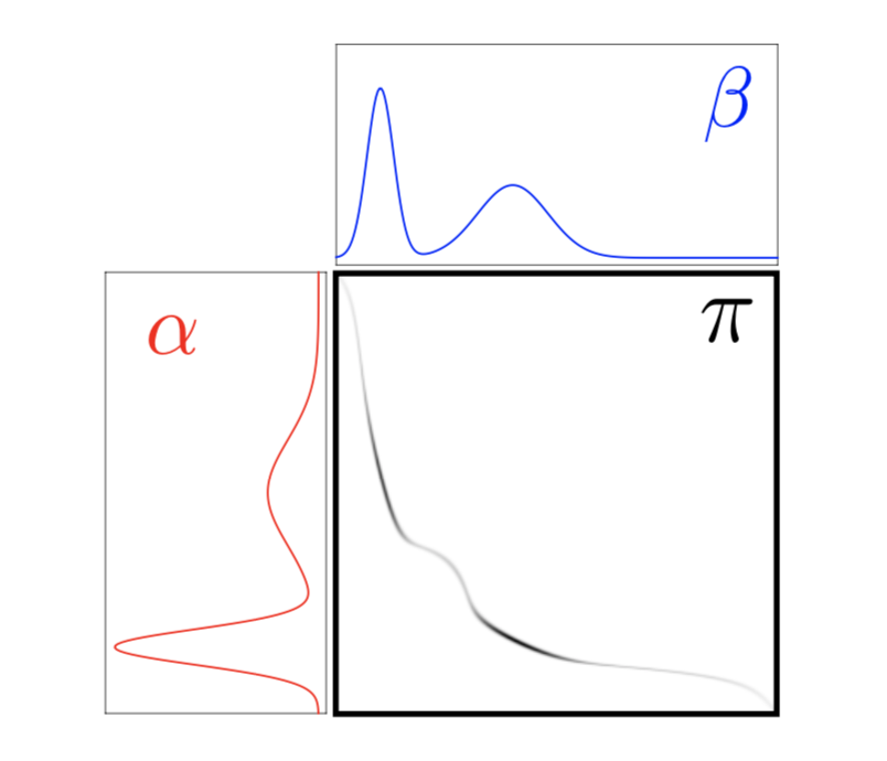
\[\mathbf{L_C} (\mathbf{a}, \mathbf{b}) \triangleq \min_{\mathbf{P} \in \mathbf{U}(\mathbf{a}, \mathbf{b})} \sum_{i,j} \mathbf{C}_{i,j} \mathbf{P}_{i,j}\]where $\mathbf{C}_{i,j} = c(x_i, y_j)$. Notice that the solution of the Kantrovich problem results in a coupling that is localized along the Monge map $(x, T(x))$ as shown below (displayed in black).
Wasserstein Distance
Consider the case of discrete probability distributions and let $n = m$ and for some $p \ge 1$, let \(\mathbf{C} = \mathbf{D}^p = \left[ \mathbf{D}_{i,j}^p \right]_{i,j} \in \mathbb{R}^{n \times n}\), where \(\mathbf{D} \in \mathbb{R}_+^{n \times n}\) is a distance on \(\mathbb{[} n \mathbb{]}\), i.e.
- \(\mathbf{D} \in \mathbb{R}_+^{n \times n}\) is symmetric.
- \(\mathbf{D}_{i,j} = 0\) if and only if \(i=j\).
- \(\forall (i,j,k) \in \mathbb{[} n \mathbb{]}^3, ~~ \mathbf{D}_{i,k} \le \mathbf{D}_{i,j} + \mathbf{D}_{j,k}\).
Then, in a non-trivial way, using Minkowski’s inequality one can prove that
\[W_p(\mathbf{a}, \mathbf{b}) \triangleq \mathbf{L}_{\mathbf{D}^p}(\mathbf{a}, \mathbf{b})^{1/p},\]is indeed a distance. This metric is called Wasserstein Distance. Notice that for the case of \(0 < p \le 1\), this is not necessarily true. In that case, \(\mathbf{D}^p\) is itself a distance and therefore \(W_p(\mathbf{a}, \mathbf{b})^p\) will be a distance on the simplex. In case of continuous domains, assuming $\mathcal{X} = \mathcal{Y}$ and $p \ge 1$ and $c(x,y) = d(x,y)^p$ for some distance $d$ on space $\mathcal{X}$, the $p$-Wasserstein distance on $\mathcal{X}$ is defined as
\[\mathcal{W}_p(\alpha, \beta) \triangleq \mathcal{L}_{d^p}(\alpha, \beta)^{1/p}\]and is similarly proved to be a distance metric.
The Wasserstein distance \(\mathcal{W}_p\) has many important properties, the most important being that it is a weak distance , i.e. it allows one to compare singular distributions (for instance, discrete ones) whose supports do not overlap and to quantify the spatial shift between the supports of two distributions. In particular, ``classical’’ distances (or divergences) are not even defined between discrete distributions (the $L^2$ norm can only be applied to continuous measures with a density with respect to a base measure, and the discrete $\ell^2$ norm requires that positions $(x_i,y_j)$ take values in a predetermined discrete set to work properly). In sharp contrast, one has that for any $p> 0$, \(\mathcal{W}_p^p(\delta_x,\delta_y) = d(x,y)\). Indeed, it suffices to notice that \(\mathcal{U}(\delta_x,\delta_y)=\{ \delta_{x,y}\}\) and therefore the Kantorovich problem having only one feasible solution, \(\mathcal{W}_p^p(\delta_x,\delta_y)\) is necessarily \((d(x,y)^p)^{1/p}=d(x,y)\). This shows that \(\mathcal{W}_p(\delta_x,\delta_y) \rightarrow 0\) if \(x \rightarrow y\). This property corresponds to the fact that $\mathcal{W}_p$ is a way to quantify weak convergence.
A nice feature of the Wasserstein distance over a Euclidean space \(\mathcal{X}=\mathbb{R}^d\) for the ground cost \(c(x,y)= \lVert x-y \lVert^2\) is that one can factor out translations; indeed, denoting \(T_{\tau} : x \mapsto x-\tau\) the translation operator, one has
\[\mathcal{W}_2(T_{\tau\sharp} \alpha,T_{\tau'\sharp} \beta)^2 = \mathcal{W}_2(\alpha,\beta)^2 - 2 \langle \tau-\tau', \mathbf{m}_{\alpha}-\mathbf{m}_{\beta} \rangle + \lVert \tau-\tau' \lVert^2,\]where \(\mathbf{m}_{\alpha} \triangleq \int_\mathcal{X} x \mathrm{d}\alpha(x) \in \mathbb{R}^d\) is the mean of $\alpha$. In particular, this implies the nice decomposition of the distance as
\[\mathcal{W}_2(\alpha,\beta)^2 = \mathcal{W}_2(\tilde\alpha,\tilde{\beta})^2 + \lVert \mathbf{m}_{\alpha}-\mathbf{m}_{\beta} \lVert^2,\]where $(\tilde\alpha,\tilde{\beta})$ are the ``centered’’ zero mean measures $\tilde\alpha=T_{\mathbf{m}_{\alpha}\sharp}\alpha$.
In case of \(p = +\infty\), the limit of $\mathcal{W}_p^p$ as \(p \rightarrow +\infty\) is
\[\mathcal{W}_{\infty}(\alpha,\beta) \triangleq \min_{\pi \in \mathcal{U}(\alpha,\beta)} \sup_{(x,y) \in \mathrm{Supp}(\pi)} d(x,y),\]where the sup should be understood as the essential supremum according to the measure $\pi$ on $\mathcal{X}^2$. In contrast to the cases $p<+\infty$, this is a nonconvex optimization problem, which is difficult to solve numerically and to study theoretically. The $\mathcal{W}_{\infty}$ distance is related to the Hausdorff distance between the supports of $(\alpha,\beta)$.
For one dimensional distributions, things become very simplified. Here is a few special cases of Wasserstein distances:
- The 1-Wasserstein distance between $\mathbf{a}$ and $\mathbf{b}$ is equal to half the 1-norm of their difference, \(\mathbf{L}_{\mathbf{C}} = \frac{1}{2} \lVert \mathbf{a} - \mathbf{b} \rVert_1\).
- For a measure $\alpha$ on $\mathbb{R}$, with the cummulative distribution function \(\mathcal{C}_{\alpha}(x)\) and quantile function \(\mathcal{C}^{-1}_{\alpha}(x)\) and for any $p \ge 1$, using a non-trivial proof (hints page 15 of here), we have
-
The above equation means that through the map $\alpha \to \mathcal{C}_{\alpha}^{-1}$, the Wasserstein distance is isometric to a linear space equipped with the $\mathbf{L}^p$ norm or, equivalently, that the Wasserstein distance for measures on the real line is a Hilbertian metric. This makes the geometry of 1-D optimal transport very simple but also very different from its geometry in higher dimensions, which is not Hilbertian.
-
For $p = 1$, we can even simplify more as
-
For $p = 1$, an optimal Monge map $T$ such that $T_{\sharp}\alpha = \beta$ is defined as \(T = \mathcal{C}^{-1}_{\beta} \circ \mathcal{C}_{\alpha}\).
-
In case of Gaussian distributions \(\alpha \sim \mathcal{N}(\mathbf{m}_{\alpha}, \mathbf{\Sigma}_{\alpha})\) and \(\beta \sim \mathcal{N}(\mathbf{m}_{\beta}, \mathbf{\Sigma}_{\beta})\), using Brenier Theorem, page 27 we can prove that the optimal Monge map is
where
\[A=\mathbf{\Sigma}_\alpha^{-\tfrac{1}{2}}\Big(\mathbf{\Sigma}_\alpha^{\tfrac{1}{2}}\mathbf{\Sigma}_\beta\mathbf{\Sigma}_\alpha^{\tfrac{1}{2}}\Big)^{\tfrac{1}{2}}\mathbf{\Sigma}_\alpha^{-\tfrac{1}{2}}=A^T\]Further,
\[\mathcal{W}_2^2( \alpha,\beta) = \lVert \mathbf{m}_\alpha - \mathbf{m}_\beta \rVert^2 + \mathcal{B}(\mathbf{\Sigma}_\alpha,\mathbf{\Sigma}_\beta)^2,\]where $\mathcal{B}$ is Bures metric , defines as
\[\mathcal{B}(\mathbf{\Sigma}_\alpha,\mathbf{\Sigma}_\beta)^2 \triangleq \mathrm{Tr} \left( \mathbf{\Sigma}_\alpha + \mathbf{\Sigma}_\beta - 2 \left( \mathbf{\Sigma}_\alpha^{\frac{1}{2}} \mathbf{\Sigma}_\beta \mathbf{\Sigma}_\alpha^{\frac{1}{2}} \right)^{\frac{1}{2}}\right)\]where $\mathbf{\Sigma}^{1/2}$ is the matrix square root. One can show that $\mathcal{B}$ is a distance on covariance matrices and that $\mathcal{B}^2$ is convex with respect to both its arguments. In the case where \(\mathbf{\Sigma}_\alpha = \mathrm{Diag}(r_i)_i\) and \(\mathbf{\Sigma}_\beta = \mathrm{Diag}(s_i)_i\) are diagonals, the Bures metric is the Hellinger distance,
\[\mathcal{B}(\mathbf{\Sigma}_\alpha,\mathbf{\Sigma}_\beta) = \lVert \sqrt{r}-\sqrt{s} \rVert_2.\]This implies that for 1-D Gaussians, $\mathcal{W}_2$ is thus the Euclidean distance on the 2-D plane plotting the mean and the standard deviation of a Gaussian.
Kantrovich Duality
The Kantorovich problem is a constrained convex minimization problem, and as such, it can be naturally paired with a so-called dual problem, which is a constrained concave maximization problem. The dual problem is of the form
\[\mathbf{L}_{\mathbf{C}}(\mathbf{a},\mathbf{b}) = \max_{(\mathbf{f},\mathbf{g}) \in \mathbf{R}(\mathbf{C})} \langle \mathbf{f}, \mathbf{a} \rangle + \langle \mathbf{g}, \mathbf{b} \rangle,\]where the set of admissible dual variables is
\[\mathbf{R}(\mathbf{C}) \triangleq \{ (\mathbf{f},\mathbf{g}) \in \mathbb{R}^n \times \mathbb{R}^m ~:~ \mathbf{f} \mathbb{1}_m^T + \mathbb{1}_n \mathbf{g} \leq \mathbf{C} \}.\]Such dual variables are often referred to as Kantorovich potentials. This result is a direct consequence of the more general result on the strong duality for linear programs and can also be achieved using Lagrangian duality. Kantrovich dual problem in case of continuous distributions will be of the form
\[\mathcal{L}_c(\alpha,\beta) = \sup_{(f,g) \in \mathcal{R}(c)}\ \int_\mathcal{X} f(x) \mathrm{d}\alpha(x) + \int_\mathcal{Y} g(y) \mathrm{d}\beta(y),\]where the set of admissible dual potentials is
\[\mathcal{R}(c) \triangleq \{(f,g) \in \mathcal{C}(\mathcal{X}) \times \mathcal{C}(\mathcal{Y}) ~~~~ \forall (x,y),~ f(x)+g(y) \leq c(x,y)\}.\]Here, $(f,g)$ is a pair of continuous functions and are also called, as in the discrete case, ``Kantorovich potentials.’’ The primal-dual optimality allows us to track the support of the optimal plan as follows
\[\mathrm{Supp}(\pi) \subset \{(x,y) \in \mathcal{X} \times \mathcal{Y} ~:~ f(x) + g(y) = c(x,y) \}\]and in case of discrete measures
\[\{(i,j) \in \mathbb{[} n \mathbb{]} \times \mathbb{[} m \mathbb{]} ~:~ \mathbf{P}_{i,j} > 0 \} \subset \{(i,j) \in \mathbb{[} n \mathbb{]} \times \mathbb{[} m \mathbb{]} ~:~ \mathbf{f}_i + \mathbf{g}_j = \mathbf{C}_{i,j} \}\]Note that in contrast to the primal problem, showing the existence of solutions to the dual problem is nontrivial, because the constraint set $\mathcal{R}(c)$ is not compact and the function to minimize noncoercive. However, in the case $c(x,y) = d(x,y)^p$ with $p \ge 1$, one can, however, show that optimal $(f,g)$ are necessarily Lipschitz regular, which enables us to replace the constraint by a compact one.
Entropic Regularization
The discrete entropy of a coupling matrix is defined as
\[\mathbf{H}(\mathbf{P}) \triangleq -\sum_{i,j} \mathbf{P}_{i,j} (\log(\mathbf{P}_{i,j})-1),\]with an analogous definition for vectors, with the convention that $\mathbf{H}(\mathbf{a}) = -\infty$ if one of the entries \(\mathbf{a}_j\) is 0 or negative. The function \(\mathbf{H}\) is 1-strongly concave, because its Hessian is \(\partial^2 \mathbf{H}(P)=-\mathrm{diag}(1/\mathbf{P}_{i,j})\) and \(\mathbf{P}_{i,j} \leq 1\). The idea of the entropic regularization of optimal transport is to use $-\mathbf{H}$ as a regularizing function to obtain approximate solutions to the original transport problem. The new optimization problem is defined as
\[\mathbf{L}_\mathbf{C}^\varepsilon(\mathbf{a},\mathbf{b}) \triangleq \min_{\mathbf{P} \in \mathbf{U}(\mathbf{a},\mathbf{b})} \langle \mathbf{P}, \mathbf{C} \rangle - \varepsilon \mathbf{H}(\mathbf{P}). \label{eq_entropic_optimization}\]Since the objective in the above optimization problem is an $\epsilon$-strongly convex function, this problem has a unique optimal solution. Let, \(\mathbf{P}_{\varepsilon}\) shows this unique solution. It can be proved that this unique solution converges to the optimal solution with maximal entropy within the set of all optimal solutions of the Kantorovich problem, namely
\[\mathbf{P}_\varepsilon \overset{\varepsilon \rightarrow 0}{\longrightarrow} \mathrm{Argmin}_{\mathbf{P}} \{ -\mathbf{H}(\mathbf{P}) ~:~ \mathbf{P} \in \mathbf{U}(\mathbf{a},\mathbf{b}), \langle \mathbf{P}, \mathbf{C} \rangle = \mathbf{L}_\mathbf{C}(\mathbf{a},\mathbf{b}) \}\]so that in particular
\[\mathbf{L}_\mathbf{C}^\varepsilon(\mathbf{a},\mathbf{b}) \overset{\varepsilon \rightarrow 0}{\longrightarrow} \mathbf{L}_\mathbf{C}(\mathbf{a},\mathbf{b}).\]One also has
\[\mathbf{P}_\varepsilon \overset{\varepsilon \rightarrow \infty}{\longrightarrow} \mathbf{a} {\mathbf{b}}^T = (\mathbf{a}_i \mathbf{b}_j)_{i,j}. \label{eq_epsilon_large}\]In other words, for a small regularization $\varepsilon$, the solution converges to the maximum entropy optimal transport coupling. In sharp contrast, for a large regularization, the solution converges to the coupling with maximal entropy between two prescribed marginals $\mathbf{a},\mathbf{b}$, namely the joint probability between two independent random variables distributed following $\mathbf{a},\mathbf{b}$.
Defining the Kullback–Leibler divergence between couplings as
\[\mathbb{KL}(\mathbf{P} \mathbb{II} \mathbf{K}) \triangleq \sum_{i,j} \mathbf{P}_{i,j} \log \left( {\frac{\mathbf{P}_{i,j}}{\mathbf{K}_{i,j}}} \right) - \mathbf{P}_{i,j} + \mathbf{K}_{i,j},\]the unique solution $\mathbf{P}_\varepsilon$ is a projection onto $\mathbf{U}(\mathbf{a},\mathbf{b})$ of the Gibbs kernel associated to the cost matrix $\mathbf{C}$ as
\[\mathbf{K}_{i,j} \triangleq e^{-\frac{\mathbf{C}_{i,j}}{\epsilon}}. \label{eq_K_sinkhorn}\]Indeed one has that using the definition above
\[\mathbf{P}_\epsilon = \mathrm{Proj}_{\mathbf{U}(\mathbf{a},\mathbf{b})}^{\mathbb{KL}}(\mathbf{K}) \triangleq \mathrm{argmin}_{\mathbf{P} \in \mathbf{U}(\mathbf{a},\mathbf{b})} \mathbb{KL} (\mathbf{P} \mathbb{II} \mathbf{K}).\]Therefore, the problem of regularized transport is that of minimizing \(\mathbf{L}_\mathbf{C}^\varepsilon(\mathbf{a},\mathbf{b})\) to find \(\mathbf{P}_\varepsilon\). This allows to define the regularized counterpart of equation \eqref{eq_kantrovich_cont} as following,
\[\mathcal{L}_c^{\epsilon} \triangleq \min_{\pi \in \mathcal{U}(\alpha, \beta)} \int_{\mathcal{X} \times \mathcal{Y}} c(x,y) \mathrm{d} \pi(x,y) + \epsilon \mathbb{KL}\left(\pi ~||~ \alpha \otimes \beta \right) \\ = \min_{(X,Y)} \left\{\mathbb{E}_{(X,Y)} \left( c(X, Y) \right) + \epsilon I(X, Y) ~:~ X \sim \alpha, ~ Y \sim \beta \right\}\]Note that if \(\epsilon \to \infty\), the optimization problem reduces to minimizing the mutual information function which results in independent distributions as expected from equation \eqref{eq_epsilon_large}. When \(\epsilon \to 0\), the solution of the regularized optimization problem converges to the solution of the optimal transport problem which is the Monge map \(Y = T(X)\) (and \(X = T^{-1}(Y)\)). In some sense, $X$ and $Y$ will be fully dependent in this case.
The dual problem for discrete distributions in case of entropic regularization will is of the form
\[\mathbf{L}_{\mathbf{C}}^{\epsilon} (\mathbf{a}, \mathbf{b}) = \max_{\mathbf{f} \in \mathbb{R}^n, ~ \mathbf{g} \in \mathbb{R}^m} \langle \mathbf{f}, \mathbf{a} \rangle + \langle \mathbf{g}, \mathbf{b} \rangle - \epsilon \langle e^{\mathbf{f}/\epsilon}, \mathbf{K} e^{\mathbf{g}/\epsilon} \rangle\]and in case of generic measures, the dual problem will be
\[\mathcal{L}_{c}^{\epsilon}(\alpha, \beta) = \sup_{(f,g) \in \mathcal{C}(\mathcal{X}) \times \mathcal{C} (\mathcal{Y})} \int_{\mathcal{X}} f \mathrm{d}\alpha + \int_{\mathcal{Y}} g \mathrm{d}\beta - \epsilon \int_{\mathcal{X} \times \mathcal{Y}} e^{\frac{1}{\epsilon}(-c(x,y)+f(x)+g(y))} \mathrm{d}\alpha(x) \mathrm{d}\beta(y)\]Sinkhorn Algorithm
It is easy to prove that the solution to the equation \eqref{eq_entropic_optimization} is unique and has the form \(\mathbf{P}_{i,j} = \mathbf{u}_i \mathbf{K}_{i,j} \mathbf{v}_j\) for \(\forall (i,j) \in \mathbb{[} n \mathbb{]} \times \mathbb{[} m \mathbb{]}\), for two unknown scaling variabls \((\mathbf{u}, \mathbf{v}) \in \mathbb{R}_+^n \times \mathbb{R}_+^m\) and $\mathbf{K}$ defined in equation \eqref{eq_K_sinkhorn}. In a matrix form, we can write \(\mathbf{P} = \mathrm{diag}(\mathbf{u}) \mathbf{K} \mathrm{diag}(\mathbf{v})\) where \(\mathrm{diag}(\mathbf{u})~ \mathbf{K} ~\mathrm{diag}(\mathbf{v})~ \mathbb{1}_m = \mathbf{a}\) and \(\mathrm{diag}(\mathbf{v}) ~\mathbf{K}^T ~\mathrm{diag}(\mathbf{u}) ~\mathbb{1}_n = \mathbf{b}\). Since \(\mathrm{diag}(\mathbf{v}) \mathbb{1}_m = \mathbf{v}\) and \(\mathrm{diag}(\mathbf{u}) \mathbb{1}_n = \mathbf{u}\), we have
\[\mathbf{u} \odot \mathbf{Kv} = \mathbf{a} \\ \mathbf{v} \odot \mathbf{K}^T\mathbf{u} = \mathbf{b}\]where $\odot$ denotes elementwise multiplication. This problem is known in the numerical analysis community as the matrix scaling problem and an intuitive way to handle these equations is to solve them iteratively, by modifying first $\mathbf{u}$ so that it satisfies the top Equation and then $\mathbf{v}$ to satisfy the buttom one. These two updates define Sinkhorn’s algorithm
\[\mathbf{u}^{l+1} \triangleq \frac{\mathbf{a}}{\mathbf{K}\mathbf{v}^l} \\ \mathbf{v}^{l+1} \triangleq \frac{\mathbf{b}}{\mathbf{K}^T\mathbf{u}^{l+1}} \label{eq_sinkhorn}\]with elementwise division and initialized with an arbitrary positive vector like \(\mathbf{v}^0 = \mathbb{1}_m\). The choice of the initial vector deos not affect convergence of the algorithm. It can be shown that the Sinkhorn iterations convergence rate is linear. It can also be implemented in to run on GPU for parallel processing.
\(\mathcal{W}_1\) Optimal Transport
Assume that \(d\) is a distance on \(\mathcal{X} = \mathcal{Y}\) and the ground cost is \(c(x,y) = d(x,y)\). Also, define the Lipschitz constant of a function \(f \in \mathcal{C}(\mathcal{X})\) as
\[Lip(f) \triangleq \sup \left\{\frac{|f(x)-f(y)|}{d(x,y)} ~:~ (x,y) \in \mathcal{X}^2, ~ x\neq y\right\}\]and define Lipschitz functions to be those functions $f$ satisfying $Lip(f) < +\infty$; they form a convex subset of $\mathcal{C}(\mathcal{X})$. Using the notion of $c$-transforms, it will not be difficult to prove that
\[\mathcal{W}_1(\alpha, \beta) = \max_f \left\{ \int_{\mathcal{X}} f(x) \mathrm{d}\alpha - \int_{\mathcal{X}} f(x) \mathrm{d}\beta ~:~ Lip(f) \le 1\right\}\]This expression shows that \(\mathcal{W}_1\) is actually a norm which is called Kantorovich and Rubinstein norm. For discrete measures $\alpha, \beta$, if we can write \(\alpha - \beta = \sum_k \mathbf{m}_k \delta_{z_k}\) for \(z_k \in \mathcal{X}\) and $\sum_k \mathbf{m}_k = 0$, then
\[\mathcal{W}_1(\alpha, \beta) = \max_{\mathbf{f}} \left\{ \sum_{k} \mathbf{f}_k \mathbf{m}_k ~:~ \forall(k,l), ~ |\mathbf{f}_k - \mathbf{f}_l| \le d(z_k, z_l)\right\}\]which is a finite-dimensional convex program with quadratic-cone constraints and can be solved using interior point methods or proximal methods. When using \(d(x,y)= \|x-y\|\) with \(\mathcal{X} = \mathbb{R}\), we can reduce the number of constraints by ordering the $z_k$’s via $z_1 \le z_2 \le \dots$ In this case, we only have to solve
\[\mathcal{W}_1(\alpha, \beta) = \max_{\mathbf{f}} \left\{ \sum_{k} \mathbf{f}_k \mathbf{m}_k ~:~ \forall k, ~ |\mathbf{f}_{k+1} - \mathbf{f}_k| \le z_{k+1} - z_k\right\}\]which is a linear program.
As mentioned before, when $0 < p \le 1$, $\tilde{d}(x,y) \triangleq d(x,y)^p$ satisfied the triangle equality and is itself a distance. Therefore, one can apply the results and algorithms above for \(\mathcal{W}_1\) on distance \(\tilde{d}(x,y)\) to compute \(\mathcal{W}_p\).
\(\mathcal{W}_1\) on Euclidean Spaces
In the special case of Euclidean spaces \(\mathcal{X} = \mathcal{Y} = \mathbb{R}^d\), using \(c(x, y) = \|x-y\|\), the global Lipschitz constraint can be made local as a uniform bound on the gradient of $f$,
\[\mathcal{W}_1(\alpha, \beta) = \max_{f} \left\{ \int_{\mathbb{R}^d} f(x) \mathrm{d} \alpha(x) - \int_{\mathbb{R}^d} f(x) \mathrm{d} \beta(x) ~:~ \|\nabla f \|_{\infty} \le 1\right\}\]here, the constraint \(\|\nabla f \|_{\infty} \le 1\) signifies that the norm of the gradient of $f$ at any point $x$ is upper bounded by 1, \(\|\nabla f \|_2 \le 1\) for any $x$. The dual problem will be an optimization problem under fixed divergence constraint
\[\mathcal{W}_1(\alpha, \beta) = \min_{s} \left\{ \int_{\mathbb{R}^d} \| s(x) \|_2 \mathrm{d}x ~:~ \mathrm{div}(s) = \alpha -\beta \right\}\]which is known as the Beckmann formulation. Here the vectorial function \(s(x) \in \mathbb{R}^2\) can be interpreted as a flow field, describing the movement of mass. Outside the support of the two input measures, $\mathrm{div}(s) = 0$, which is the conservation of mass constraint.
Statistical Divergences
A divergence $D$ typically satisfies $D(\alpha, \beta) \ge 0$ and $D(\alpha, \beta) = 0$ if and only if $\alpha = \beta$, but it does not need to be symmetric or satisfy the triangular inequality. Divergences are functionals which, by looking at the pointwise ratio between two measures, give a sense of how close they are